Three waveforms for synaptic conductance: (a) single exponential decay with τ = 3 ms, (b) alpha function with τ = 1 ms, and (c) dual exponential with τ1 = 3 ms and τ2 = 1 ms. Response to a single presynaptic action potential arriving at time=1ms. All conductances are scaled to a maximum of 1 (arbitrary units).
Figure 7.all

Synaptic conductance waveforms
Simulation environment:
Download:
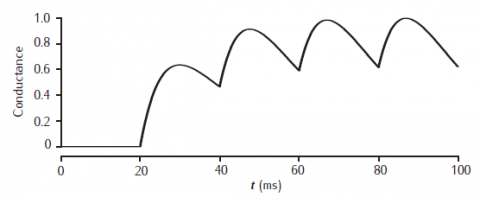
Train of synaptic waveforms
Alpha function conductance with τ = 10 ms responding to action potentials occurring at 20, 40, 60 and 80 ms. Conductance is scaled to a maximum of 1 (arbitrary units).
Simulation environment:
Download:
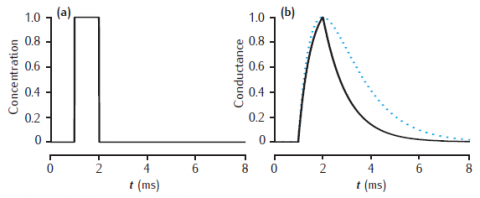
2-gate kinetic receptor model
Response of the simple 2-gate kinetic receptor model to a single pulse of neurotransmitter of amplitude 1 mM and duration1 ms. Rates are α = 1 /mM.ms and β = 1 /ms. Conductance waveform scaled to an amplitude of 1 and compared with an alpha function with τ = 1 ms (dotted line).
Simulation environment:
Download:
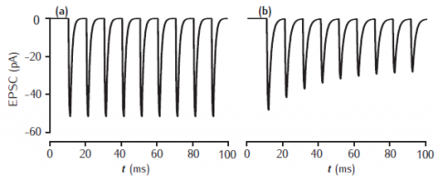
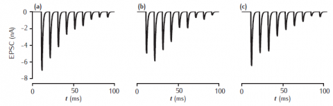
Postsynaptic EPSCs due to 2- and 5-gate AMPA receptor kinetic models
Postsynaptic current in response to 100Hz stimulation from (a) 2-gate kinetic receptor model, α = 4 /mM.ms, β = 1 /ms; (b) 5-gate desensitising model, Rb = 13 /mM.ms, Ru1 = 0.3 /ms, Ru2 = 200 /ms, Rd = 10 /ms, Rr = 0.02 /ms, Ro = 100 /ms, Rc = 1 /ms. Each presynaptic action potential is assumed to result in the release of a vesicle of neurotransmitter, giving a square-wave transmitter pulse amplitude of 1 mM and duration of 1 ms. The current is calculated as Isyn(t) = gsyn(t)(V(t) − Esyn). Esyn = 0 mV and the cell is clamped at −65 mV. The value of gsyn(t) approaches 0.8 nS on the first pulse.
Simulation environment:
Download:

Facilitation of release probability
Facilitation of release probability in the basic phenomenological model. Stimulation at 50Hz with p0 = 0.1, dp = 0.1 and τf = 100 ms.
Simulation environment:
Download:
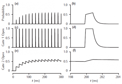
Facilitation of transmitter release in a kinetic 2-gate model
Facilitation of transmitter release in a kinetic 2-gate model. Left-hand column shows stimulation at 50 Hz. Right-hand column shows release and gating transients at the tenth pulse. Fast gate: k+1 = 200 /mM.ms, k−1 = 3 /ms; Slow gate: k+2 = 0.25 /mM.ms, k−2 = 0.01 /ms; square-wave [Ca2+]r pulse: 1 mM amplitude, 1 ms duration.
Simulation environment:
Download:
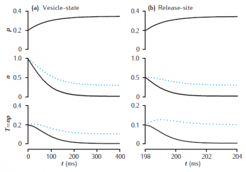
Deterministic models of short-term synaptic dynamics
Facilitation and depression in deterministic models of short-term synaptic dynamics. Phenomenological model of facilitation: p0 = 0.2; Δp = 0.05; τf = 100 ms. (a) vesicle-state model: k∗n = kr = 0.2 /s. (b) release-site model: nT = 1; kn = kr = 0.2 /s. Solid lines: ns = 0; dotted lines: ns = 0.1. Synapse stimulated at 50Hz.
Simulation environment:
Notes
Unzip file and run runsynnp_rv.m in MATLAB.
Download:
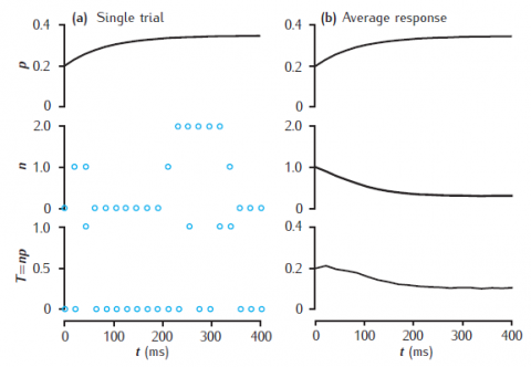
Stochastic model of short-term synaptic dynamics
Stochastic vesicle-state model of short-term dynamics at a single synaptic active zone. (a) A single simulation run, showing the release probability p, the actual number of releasable vesicles, n (initially 1), and neurotransmitter release, T. (b) Average values of these variables, taken over 10000 trials. Phenomenological model of facilitation: p0 = 0.2; Δp = 0.05; τf = 100 ms. Vesicle-state model: k∗n = kr = 0.2 s−1; ns = 0.1. Synapse stimulated at 50Hz.
Simulation environment:
Notes
Unzip file and run runsynnp_rvs.m in MATLAB. Results may not be identical to the figure as this is a stochastic model and the results depend on the random number generator and its seed.
Download:
Complete stochastic synapse model
Three distinct trials of a complete synapse model with 500 independent active zones. Each active zone uses the stochastic vesicle-state model of short-term synaptic dynamics combined with the 2-gate kinetic model of AMPA receptors. Phenomenological model of facilitation: p0 = 0.2; Δp = 0.05; τf = 100 ms. Vesicle-state model: k∗n = kr = 0.2 s−1; ns = 0. 2-gate kinetic receptor model: α = 4 mM−1ms−1, β = 1 ms−1. Esyn = 0 mV, with postsynaptic cell clamped at −65 mV. Synapse stimulated at 100Hz.
Simulation environment:
Notes
A different result appears each time you run the simulation, since it is a stochastic model.
Download:
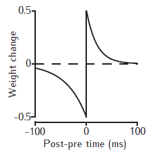
STDP weight change curve
Example STDP weight change curves. The weight is increased if the postsynaptic spike occurs at the time of, or later than the presynaptic spike; otherwise the weight is decreased. The magnitude of the weight change decreases with the time interval between the pre- and postsynaptic spikes. No change occurs if the spikes are too far apart in time.
Simulation environment:
Download:
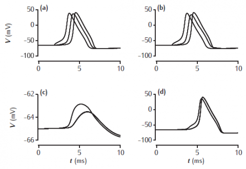
Axon gap junction model
Simulated action potential travelling along two axons that are joined by a gap junction half-way along their length. Membrane potentials are recorded at the start, middle and end of the axons. (a,b) Axon in which an action potential is initiated by a current injection into one end. (c) Other axon, with a 1 nS gap junction. (d) Other axon, with a 10 nS gap junction. Axons are 100 μm long, 2 μm in diameter with standard Hodgkin-Huxley sodium, potassium and leak channels.
Simulation environment:
Notes
Set value of r in both Ggap panels to appropriate value. This resistance is in MOhms, so 100 MOhms is 10 nS and 1000 MOhms is 1 nS.
Download: