Our simulations of a network of recurrently connected excitatory and inhibitory neurons using Equations 9.3, 9.4 and 9.5, after Amit and Brunel (1997b). (a-c) The time courses of the membrane potential of three excitatory neurons. (d) The time course of one inhibitory neuron. (e) A spike raster of 60 excitatory neurons (lower traces) and 15 inhibitory neurons (upper traces, highlighted in blue). (f ) Population firing rates of the excitatory (black) and inhibitory neurons (blue). (g) Average autocorrelation of spikes from excitatory neurons. (h) Histogram of average firing rates of excitatory neurons (black) and inhibitory neurons (blue). Parameter values: θ = 20mV, Vreset = 10mV, τE = 10ms, τI = 5ms, wEE = 0.21 V s-1, wEI = 0.63 V s-1, wIE = 0.35 Vs-1, wII = 1.05 V s-1, Δ=0.1, τij is drawn uniformly from the range [0.5,1.5] ms and νextE = 13Hz.
Figure 9.8
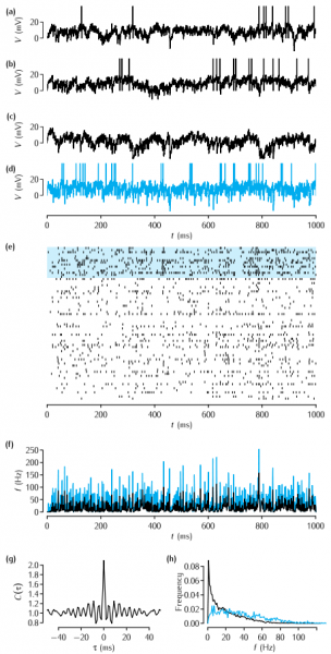
Simulations of a network of recurrently connected excitatory and inhibitory neurons after Amit and Brunel (1997b).
Simulation environment:
Notes
To run this simulation, click on the Run button in the Control panel. The simulation is quite slow compared to others from this website - it will probably take a few minutes to run. The scale value in the Control panel indicates how big the network is compared to the one simulated in the book. The default is 0.5, i.e. there are half as many exicitatory and inhibitory neurons as in the simulations used to produce the figure in the book.
Download: