Code examples
Chapter 1
Figure 1.1
[img_assist|nid=15|title=Figure 1.1|desc=|link=none|align=right|width=242|height=300]
Here is some code that reproduces figure 1.
Instructions. Start R and then type:
> source("figures.R")
Chapter 2
Chapter 3
Chapter 4
Effect of spines on somatic voltage response
Somatic voltage response to a single synaptic EPSP on a spine at a distance of 500 μm in the apical dendrites of a CA1 pyramidal cell model (blue dot on cell image). The voltage amplitude is reduced (black line) when 20,000 inactive spines are evenly distributed in the dendrites, compared to when no spines are included (blue dashed line). The somatic voltage response is corrected if Rm is decreased and Cm is increased in proportion with the additional membrane area due to spines
(blue dotted line). The CA1 pyramidal cell is n5038804, as used in Migliore et al. (2005); model has 455 compartments (with no spines); passive membrane throughout with Rm = 28 kΩ cm2, Ra = 150 Ω cm, Cm = 1 μF cm−2; spine head: diameter 0.5 μm, length 0.5 μm; spine neck: diameter 0.2 μm, length 0.5 μm; 20,000 spines increase the total membrane area by 1.4 and reduce the somatic voltage response by around 30%. For a similar comparison see Holmes and Rall (1992b).
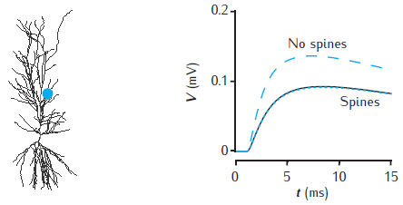
Simulation starts with no spines. Use the "Control" panel (which may initially be hidden behind other windows) to add and delete spines, or to adjust membrane resistance and capacitance to compensate for spines. Note that adding spines may take several minutes and the subsequent simulation runs more slowly.
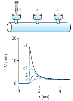
Spines on a dendrite
Voltage response to a single synaptic EPSP at a spine on a dendrite. There are three spines 100 μm apart on a 1000 μm long dendrite of 2 μm diameter. EPSP occurs at spine 1. Black lines show the voltage at each spine head. Blue lines are the voltage response in the dendrite at the base of each spine. Dendrite modelled with 1006 compartments (1000 for main dendrite plus 2 for each spine); passive membrane throughout with Rm = 28 kΩ cm2, Ra = 150 Ω cm, Cm = 1 μF cm−2; spine head: diameter 0.5 μm, length 0.5 μm; spine neck: diameter 0.2 μm, length 0.5 μm. For a similar circuit see Woolf et al. (1991).
Chapter 5
Chapter 6
Calcium transients for different numbers of shells
Calcium transients in the (a) submembrane shell and (b) cell core (central shell) for different total numbers of shells. Black line: 11 shells. Gray dashed line: 4 shells. Blue dotted line: 2 shells. Diameter is 4 μm and the submembrane shell is 0.1 μm thick. Other shells equally subdivide the remaining compartment radius. All other model parameters are as in Figure 6.5.

Note that the simulation plots correctly show the calcium transients all beginning after the stimulus at 20 msecs, unlike the figure in the book in which part (b) has a spurious time shift! (This is a drawing error, not a simulation error).
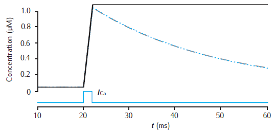
Calcium transients in a cylindrical compartment
Calcium transients in a 1.0 single cylindrical compartment, 1 μm in diameter and 1 μm in length (similar in size to a spine head). Initial concentration is 0.05 μM. Influx is due to a calcium current of 5 μA cm−2, starting at 20 ms for 2 ms, across the radial surface. Black line: accumulation of calcium with no decay or extrusion. Blue line: simple decay with τdec = 27 ms. Gray dashed line: instantaneous pump with Vpump = 4 × 10⁻⁶ μMs−1, equivalent to 10−11 mol cm−2 s−1 through the surface area of this compartment, Kpump = 10 μM, Jleak = 0.0199 × 10⁻⁶ μMs−1.
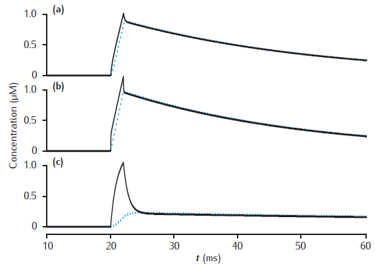
Calcium transients in a submembrane shell
Calcium transients in the submembrane shell (black lines) and the compartment core (blue dashed lines) of a two pool model that includes a membrane-bound pump and diffusion into the core. Initial concentration Ca0 is 0.05 μM throughout. Calcium current as in Figure 6.3. Compartment length is 1 μm. (a) Compartment diameter is 1 μm, shell thickness is 0.1 μm; (b) Compartment diameter is 1 μm, shell thickness is 0.01 μm; (c) Compartment diameter is 4 μm, shell thickness is 0.1 μm. Diffusion: DCa = 2.3 × 10⁻⁶ cm2 s−1; Pump: Vpump = 10−11 mol cm−2 s−1, Kpump = 10 μM, Jleak = Vpump ∗ Ca0/(Kpump + Ca0).
Calcium transients in a three pool model
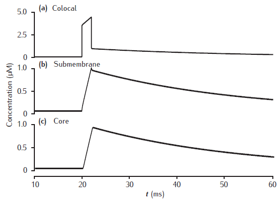
Calcium transients in (a) the potassium channel colocalised pool, (b) the larger submembrane shell, (c) the compartment core in a three pool model. Note that in (a) the concentration is plotted on a different scale. Compartment 1 μm in diameter with 0.1 μm thick submembrane shell; colocalised membrane occupies 0.001% of the total membrane surface area. Calcium influx into the colocalised pool. Calcium current, diffusion and membrane-bound pump parameters as in Figure 6.5.
Calcium transients with slow buffer
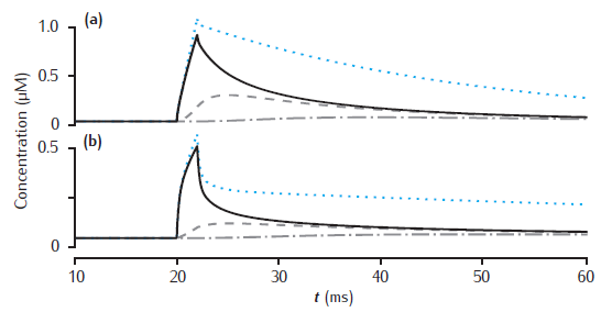
Calcium transients in (a) the 0.1 μm thick submembrane shell and (b) the cell core of a single dendritic compartment of 4 μm diameter with 4 radial shells. Slow buffer with initial concentration 50 μM, forward rate k+ = 1.5 μM-1s−1 and backward rate k− = 0.3 s−1. Blue dotted line: unbuffered calcium transient. Gray dashed line (hidden by solid line): excess (EBA) approximation. Gray dash-dotted line: rapid (RBA) buffer approximation. Binding ratio κ = 250. All other model parameters as in Figure 6.5.
Use Parameters panel in GUI to change parameter values for buffered model, EBA and RBA simultaneously. Same code can generate results for both figures 6.12 and 6.13.
Longitudinal diffusion of calcium
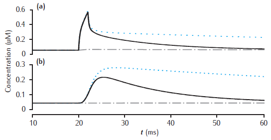
Longitudinal diffusion along a 10 μm length of dendrite. Plots show calcium transients in the 0.1 μm thick submembrane shell at different positions along the dendrite. Solid black line: 0.5 μm; dashed: 1.5 μm; dot-dashed: 4.5 μm. (a) Diameter is 1 μm. (b) Diameter is 4 μm. Calcium influx occurs in the first 1 μm length of dendrite only. Each of ten 1 μm long compartment contains four radial shells. Blue dotted line: calcium transient with only radial (and not longitudinal) diffusion in the first 1 μm long compartment. All other model parameters as in Figure 6.5.
Simulation does not reproduce calcium transient without longitudinal diffusion (blue dotted line in figure).
Michaelis-Menten kinetics
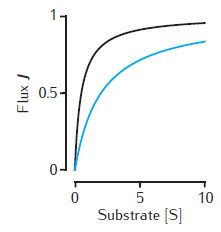
Two examples of the enzymatic flux, J, as a function of the substrate concentration, [S], for Michaelis-Menten kinetics (Equation 6.1). Arbitrary units are used and Vmax = 1. Black line: Km = 0.5. Blue line: Km = 2. Note that half-maximal flux occurs when [S] = Km.
Chapter 7
2-gate kinetic receptor model
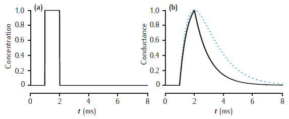
Response of the simple 2-gate kinetic receptor model to a single pulse of neurotransmitter of amplitude 1 mM and duration1 ms. Rates are α = 1 /mM.ms and β = 1 /ms. Conductance waveform scaled to an amplitude of 1 and compared with an alpha function with τ = 1 ms (dotted line).
Axon gap junction model
Simulated action potential travelling along two axons that are joined by a gap junction half-way along their length. Membrane potentials are recorded at the start, middle and end of the axons. (a,b) Axon in which an action potential is initiated by a current injection into one end. (c) Other axon, with a 1 nS gap junction. (d) Other axon, with a 10 nS gap junction. Axons are 100 μm long, 2 μm in diameter with standard Hodgkin-Huxley sodium, potassium and leak channels.

Set value of r in both Ggap panels to appropriate value. This resistance is in MOhms, so 100 MOhms is 10 nS and 1000 MOhms is 1 nS.
Complete stochastic synapse model
Three distinct trials of a complete synapse model with 500 independent active zones. Each active zone uses the stochastic vesicle-state model of short-term synaptic dynamics combined with the 2-gate kinetic model of AMPA receptors. Phenomenological model of facilitation: p0 = 0.2; Δp = 0.05; τf = 100 ms. Vesicle-state model: k∗n = kr = 0.2 s−1; ns = 0. 2-gate kinetic receptor model: α = 4 mM−1ms−1, β = 1 ms−1. Esyn = 0 mV, with postsynaptic cell clamped at −65 mV. Synapse stimulated at 100Hz.
A different result appears each time you run the simulation, since it is a stochastic model.
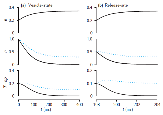
Deterministic models of short-term synaptic dynamics
Facilitation and depression in deterministic models of short-term synaptic dynamics. Phenomenological model of facilitation: p0 = 0.2; Δp = 0.05; τf = 100 ms. (a) vesicle-state model: k∗n = kr = 0.2 /s. (b) release-site model: nT = 1; kn = kr = 0.2 /s. Solid lines: ns = 0; dotted lines: ns = 0.1. Synapse stimulated at 50Hz.
Unzip file and run runsynnp_rv.m in MATLAB.
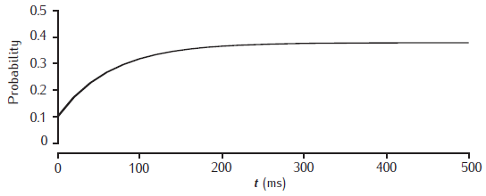
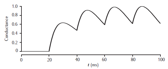
Facilitation of release probability
Facilitation of release probability in the basic phenomenological model. Stimulation at 50Hz with p0 = 0.1, dp = 0.1 and τf = 100 ms.
Facilitation of transmitter release in a kinetic 2-gate model
Facilitation of transmitter release in a kinetic 2-gate model. Left-hand column shows stimulation at 50 Hz. Right-hand column shows release and gating transients at the tenth pulse. Fast gate: k+1 = 200 /mM.ms, k−1 = 3 /ms; Slow gate: k+2 = 0.25 /mM.ms, k−2 = 0.01 /ms; square-wave [Ca2+]r pulse: 1 mM amplitude, 1 ms duration.
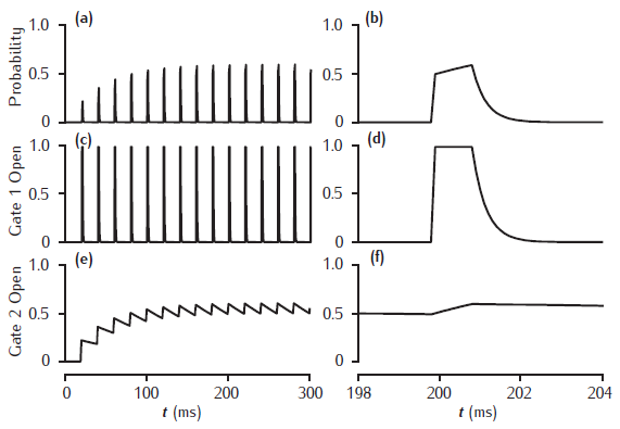
Figure 7.2
Here is some Matlab code that reproduces Figure 7.2[img_assist|nid=19|title=Figure 7.2|desc=Synaptic conductance waveforms|link=none|align=right|width=370|height=113]
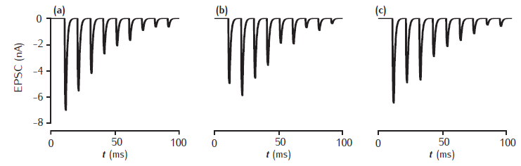
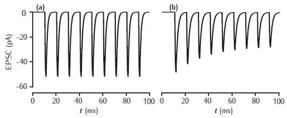
Postsynaptic EPSCs due to 2- and 5-gate AMPA receptor kinetic models
Postsynaptic current in response to 100Hz stimulation from (a) 2-gate kinetic receptor model, α = 4 /mM.ms, β = 1 /ms; (b) 5-gate desensitising model, Rb = 13 /mM.ms, Ru1 = 0.3 /ms, Ru2 = 200 /ms, Rd = 10 /ms, Rr = 0.02 /ms, Ro = 100 /ms, Rc = 1 /ms. Each presynaptic action potential is assumed to result in the release of a vesicle of neurotransmitter, giving a square-wave transmitter pulse amplitude of 1 mM and duration of 1 ms. The current is calculated as Isyn(t) = gsyn(t)(V(t) − Esyn). Esyn = 0 mV and the cell is clamped at −65 mV. The value of gsyn(t) approaches 0.8 nS on the first pulse.
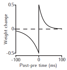
STDP weight change curve
Example STDP weight change curves. The weight is increased if the postsynaptic spike occurs at the time of, or later than the presynaptic spike; otherwise the weight is decreased. The magnitude of the weight change decreases with the time interval between the pre- and postsynaptic spikes. No change occurs if the spikes are too far apart in time.
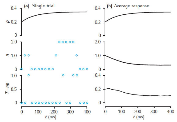
Stochastic model of short-term synaptic dynamics
Stochastic vesicle-state model of short-term dynamics at a single synaptic active zone. (a) A single simulation run, showing the release probability p, the actual number of releasable vesicles, n (initially 1), and neurotransmitter release, T. (b) Average values of these variables, taken over 10000 trials. Phenomenological model of facilitation: p0 = 0.2; Δp = 0.05; τf = 100 ms. Vesicle-state model: k∗n = kr = 0.2 s−1; ns = 0.1. Synapse stimulated at 50Hz.
Unzip file and run runsynnp_rvs.m in MATLAB. Results may not be identical to the figure as this is a stochastic model and the results depend on the random number generator and its seed.
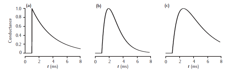
Synaptic conductance waveforms
Three waveforms for synaptic conductance: (a) single exponential decay with τ = 3 ms, (b) alpha function with τ = 1 ms, and (c) dual exponential with τ1 = 3 ms and τ2 = 1 ms. Response to a single presynaptic action potential arriving at time=1ms. All conductances are scaled to a maximum of 1 (arbitrary units).
Chapter 8
Chapter 9
Biophysical associative memory model
Network simulation based on the model of Sommer and Wennekers (2001). The top three traces are the time courses of the membrane potential of three excitatory neurons: (a) a cue cell, (b) a pattern cell and (c) a non-pattern cell. (d) a spike raster of the 100 excitatory neurons. (e) the recall quality over time, with a sliding 10ms time window.
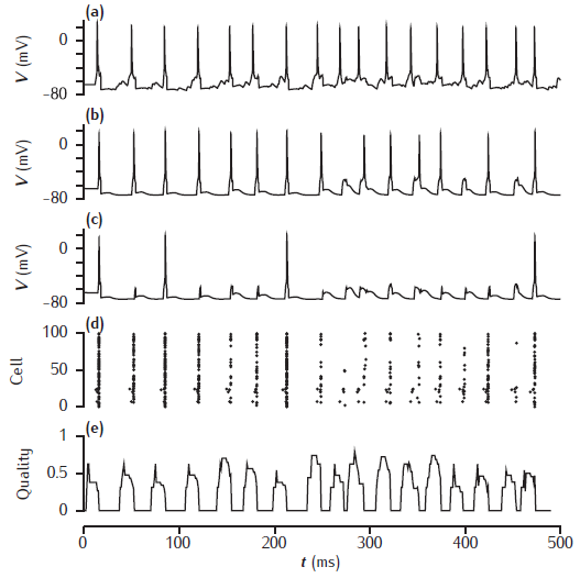
Simulation produces somatic voltage plots from a cue cell, a non-cue pattern cell and a non-pattern cell. The "Spike plot" button on the menu panel will show a raster plot of all spiking activity during the simulation.
Chapter 10
Elongation of a model neurite
Elongation of a model neurite over time in three growth modes (McLean and Graham, 2004; Graham et al., 2006). Achieved steady-state lengths are stable in each case, but there is a prominent overshoot and retraction before reaching steady state in the moderate growth mode.
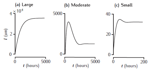
Unzip the file and run CMNG_main.m in Matlab. It takes a little while to run the simulations before plotting the results.