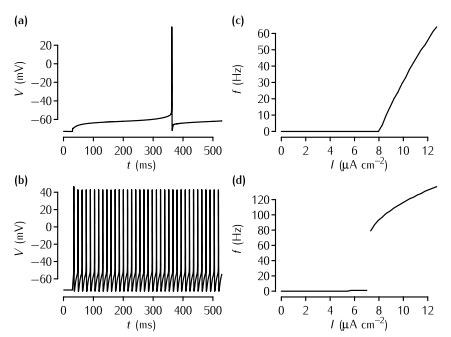
The effect of the A-type current on neuronal firing in simulations. (a) The time course of the membrane potential in the model described in Box 5.2 in response to current injection of 8.21 µA cm2 that is just superthreshold. The delay from the start of the current injection to the neuron firing is over 300 ms. (b) The response of the model to a just suprathreshold input (7.83 µA cm2) when the A-type current is removed. The spiking rate is much faster. In order to maintain a resting potential similar to the neuron with the A-type current, the leak equilibrium potential EL is set to -72.8 mV in this simulation. (c) A plot of firing rate f versus input current I in the model with the A-type conductance shown in (a). Note the gradual increase of the firing rate just above the threshold, the defining characteristic of Type I neurons. (d) The f-I plot of the neuron with no A-type conductance shown in (b). Note the abrupt increase in firing rate, the defining characteristic of Type II neurons.
Figure 5.all
Once the simulation file is open, these are the steps to reproduce each figure:
Panel (a)
- In the top Parameters window, click on the checkbox next to Type I parameters
- Click on Set Type I threshold current
- Click on Init & Run in the Run Control window
Panel (b)
- In the top Parameters window, click on the checkbox next to Type II parameters
- Click on Set Type II threshold current
- Click on Init & Run in the Run Control window
Panel (c)
- In the top Parameters window, click on the checkbox next to Type I parameters
- Click on Plot in the Grapher window
- Simulations for a number of levels of current injection will be run and the firing frequency will be plotted against current in the Grapher window.
- Once the simulations have run, to make sure you can see these results, right-click in this graph area and select View... -> View = Plot
Panel (d)
As for panel (c), except in step 1, click on the checkbox next to Type II parameters.
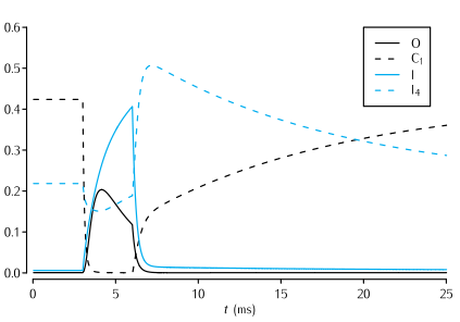
Time evolution of a selection of the state variables in the Vandenberg and Bezanilla (1991) model of the sodium channel in response to a 3 ms long voltage pulse from -65 mV to -20 mV, and back to -65 mV. See Scheme 5.7 for the significance of the state variables shown. In the interests of clarity, only the evolution of the state variables I, O, I4 and C1 are shown.
To reproduce the simulation:
- In the I/V Electrode window click on the VClamp checkbox
- In the Run Control window click on Init & Run
To view the channel's kinetic scheme, in the ChannelBuild[0] window click on highlighted text O: 9 state, 9 transitions.
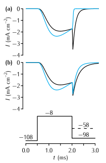
Tail currents in the Vandenberg and Bezanilla (1991) model (VB, black traces) and the Hodgkin and Huxley (1952d) model (HH, blue traces) of the sodium current in squid giant axon in response to the voltage-clamp protocol shown at the base, where the final testing potential could be (a) -98mV or (b) -58mV. During the testing potential, the tail currents show a noticeably slower rate of decay in the VB model than in the HH model. To assist comparison, the conductance in the VB model was scaled so as to make the current just before the tail current the same as in the HH model. Also, a quasi-ohmic I-V characteristic with the same ENa as the HH model was used rather than the GHK I-V characteristic used in the VB model. This does not affect the time constants of the currents, since the voltage during each step is constant.
This simulation contains two separate neurons, one containing VB model sodium channels and one containing HH model sodium channels. The parameters of each neuron are described in the windows entitled somavb and somahh. Each neuron has a voltage clamp electrode inserted.
To reproduce panel (a):
- In both I/V Clamp Electrode windows click on the checkbox next to VClamp
- In the Run Control window click on Init & Run
- The currents shown in Fig 5.13a should appear in the middle graph on the right. Additionally, the upper graph shows the states of the VB channel (see Fig 5.12) and the lower graph shows the conductance of the two types of channels
To reproduce panel (b)
- In both I/V Clamp Electrode windows in the Return Level section change the amplituce to -58mV
- In the Run Control window click on Init & Run
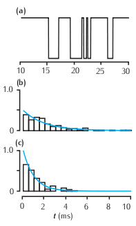
Features of a two-state kinetic scheme. (a) Simulated sample of the time course of channel conductance of the kinetic scheme described in Scheme (5.13). The parameters are α = 1 ms-1 and β = 0.5 ms-1. (b) Histogram of the open times in a simulation and the theoretical prediction of 0.5e-0.5t from Equation 5.14. (c) Histogram of the simulated closed times and the theoretical prediction e-t.
To run the simulation:
- In the Run Control window click on Init & Run
- In the top graph a trace of the conductance of the channel should appear. In the middle and lower graphs histogram of the open and closed time distributions with theoretical predictions should appear.
To change the rate of the opening and closing:
- In the ChannelBuild[0] window click on O: 2 state, 1 transitions
- In the ChannelBuildGateGUI window that opens, change the values in the boxes at the lower right. The forward rate (α in the figure) is aCO and the backard rate β is aCO.
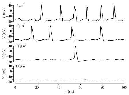
Simulations of patches of membrane of various sizes with stochastic Na+ and K+ channels. The density of Na+ and K+ channels is 60 channels per µm2 and 18 channels per µm2 respectively, and the single channel conductance of both types of channel γ = 2 pS. The Markov kinetic scheme versions of the Hodgkin-Huxley potassium and sodium channel models were used (Schemes 5.5 and 5.8). The leak conductance and capacitance is modelled as in the standard HH model. No current is applied; the action potentials are due to the random opening of a number of channels taking the membrane potential to above threshold.
To produce a trace similar to the top trace in the figure:
- In the Run Control window click on Init & Run.
- A trace similar to the top one in the figure will appear in the top right graph. Below this is a graph of the sodium and potassium currents.
To reproduce each of the other panels from the figure:
- In the soma window change the length L of the soma to the area of membrane you wish to simulate. Since the diameter of the neuron is 1/π the neuron's area in µm2 is equal to its length in µm.
- In the PointProcessGroupManager window click on nahh[0]. In the panel on the right set Nsingle to 18 multiplied by the area in µm2. For example if the area is 10µm2, Nsingle should be 180. This step is necessary because the NEURON PointProcess describes the number of channels inserted rather than their density. To maintain a constant density, the number of channels has to be scaled in line with the area.
- In the PointProcessGroupManager window click on khh[0]. In the panel on the right set Nsingle to 60 multiplied by the area in µm2. For example if the area is 10µm2, Nsingle should be 600.
- In the Run Control window click on Init & Run. Traces should appear as above.
To investigate the kinetic schems of the sodium and potassium channels:
- In the ChannelBuild[0] window click on O: 8 state, 10 tranisitions. This shows the sodium kinetic scheme.
- In the ChannelBuild[1] window click on O: 5 state, 4 tranisitions. This shows the potassium kinetic scheme.