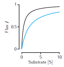
Two examples of the enzymatic flux, J, as a function of the substrate concentration, [S], for Michaelis-Menten kinetics (Equation 6.1). Arbitrary units are used and Vmax = 1. Black line: Km = 0.5. Blue line: Km = 2. Note that half-maximal flux occurs when [S] = Km.
Figure 6.all
Michaelis-Menten kinetics
Simulation environment:
Download:
Calcium transients in a cylindrical compartment
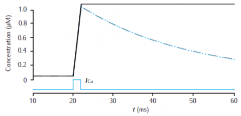
Calcium transients in a 1.0 single cylindrical compartment, 1 μm in diameter and 1 μm in length (similar in size to a spine head). Initial concentration is 0.05 μM. Influx is due to a calcium current of 5 μA cm−2, starting at 20 ms for 2 ms, across the radial surface. Black line: accumulation of calcium with no decay or extrusion. Blue line: simple decay with τdec = 27 ms. Gray dashed line: instantaneous pump with Vpump = 4 × 10⁻⁶ μMs−1, equivalent to 10−11 mol cm−2 s−1 through the surface area of this compartment, Kpump = 10 μM, Jleak = 0.0199 × 10⁻⁶ μMs−1.
Simulation environment:
Download:
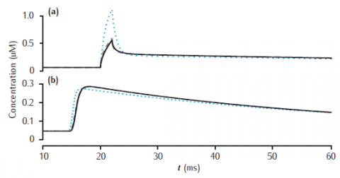
Calcium transients in a submembrane shell
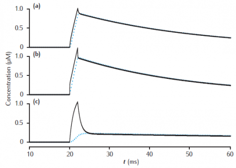
Calcium transients in the submembrane shell (black lines) and the compartment core (blue dashed lines) of a two pool model that includes a membrane-bound pump and diffusion into the core. Initial concentration Ca0 is 0.05 μM throughout. Calcium current as in Figure 6.3. Compartment length is 1 μm. (a) Compartment diameter is 1 μm, shell thickness is 0.1 μm; (b) Compartment diameter is 1 μm, shell thickness is 0.01 μm; (c) Compartment diameter is 4 μm, shell thickness is 0.1 μm. Diffusion: DCa = 2.3 × 10⁻⁶ cm2 s−1; Pump: Vpump = 10−11 mol cm−2 s−1, Kpump = 10 μM, Jleak = Vpump ∗ Ca0/(Kpump + Ca0).
Simulation environment:
Download:
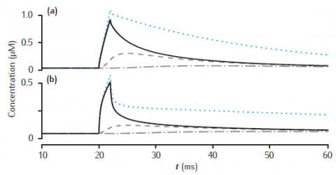
Calcium transients in a three pool model
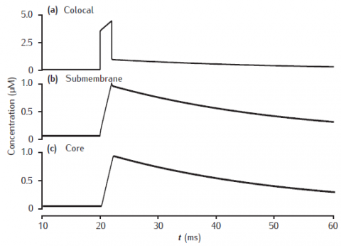
Calcium transients in (a) the potassium channel colocalised pool, (b) the larger submembrane shell, (c) the compartment core in a three pool model. Note that in (a) the concentration is plotted on a different scale. Compartment 1 μm in diameter with 0.1 μm thick submembrane shell; colocalised membrane occupies 0.001% of the total membrane surface area. Calcium influx into the colocalised pool. Calcium current, diffusion and membrane-bound pump parameters as in Figure 6.5.
Simulation environment:
Download:
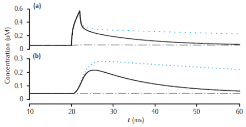
Calcium transients for different numbers of shells
Calcium transients in the (a) submembrane shell and (b) cell core (central shell) for different total numbers of shells. Black line: 11 shells. Gray dashed line: 4 shells. Blue dotted line: 2 shells. Diameter is 4 μm and the submembrane shell is 0.1 μm thick. Other shells equally subdivide the remaining compartment radius. All other model parameters are as in Figure 6.5.
Simulation environment:
Notes
Note that the simulation plots correctly show the calcium transients all beginning after the stimulus at 20 msecs, unlike the figure in the book in which part (b) has a spurious time shift! (This is a drawing error, not a simulation error).
Download:
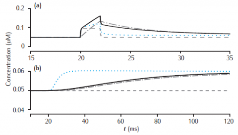
Longitudinal diffusion of calcium
Longitudinal diffusion along a 10 μm length of dendrite. Plots show calcium transients in the 0.1 μm thick submembrane shell at different positions along the dendrite. Solid black line: 0.5 μm; dashed: 1.5 μm; dot-dashed: 4.5 μm. (a) Diameter is 1 μm. (b) Diameter is 4 μm. Calcium influx occurs in the first 1 μm length of dendrite only. Each of ten 1 μm long compartment contains four radial shells. Blue dotted line: calcium transient with only radial (and not longitudinal) diffusion in the first 1 μm long compartment. All other model parameters as in Figure 6.5.
Simulation environment:
Notes
Simulation does not reproduce calcium transient without longitudinal diffusion (blue dotted line in figure).
Download:
Calcium transients with slow buffer
Calcium transients in (a) the 0.1 μm thick submembrane shell and (b) the cell core of a single dendritic compartment of 4 μm diameter with 4 radial shells. Slow buffer with initial concentration 50 μM, forward rate k+ = 1.5 μM-1s−1 and backward rate k− = 0.3 s−1. Blue dotted line: unbuffered calcium transient. Gray dashed line (hidden by solid line): excess (EBA) approximation. Gray dash-dotted line: rapid (RBA) buffer approximation. Binding ratio κ = 250. All other model parameters as in Figure 6.5.
Simulation environment:
Notes
Use Parameters panel in GUI to change parameter values for buffered model, EBA and RBA simultaneously. Same code can generate results for both figures 6.12 and 6.13.
Download:
Calcium transients with fast buffer
Calcium transients in (a) the 0.1 μm thick submembrane shell and (b) the cell core of a single dendritic compartment of 4 μm diameter with 4 radial shells. Fast buffer with initial concentration 50 μM, forward rate k+ = 500 μM-1s−1 and backward rate k− = 1000 s−1. Black solid line: fixed buffer. Blue dotted line: mobile buffer with diffusion rate Dbuf = 1 × 10⁻⁶ cm2 s−1. Gray dashed line: excess (EBA) approximation. Gray dash-dotted line: rapid (RBA) buffer approximation. Binding ratio κ = 25. All other model parameters as in Figure 6.5.
Simulation environment:
Notes
Use Parameters panel to change all parameter values. Code produces results for figures 6.12 and 6.13.
Download: