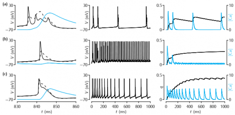
Behaviour of the Pinsky-Rinzel model for different values of the coupling parameter gc and the level of somatic current injection Is. In each subfigure, the left-hand column shows the detail of the somatic membrane potential (solid line), the dendritic membrane potential (dashed line) and the calcium concentration (blue line) in a period of 30 ms around a burst or action potential. The middle column shows the behaviour of the membrane potential over 1000 ms. The right-hand column shows the behaviour of q, the IAHP activation variable, and the calcium concentration over the period of 1000 ms. The values of Is in mA cm-2 and gc in mS cm-2 in each row are: (a) 0.15, 2.1; (b) 0.50, 2.1; (c) 0.50, 10.5.
Figure 8.all
Pinsky-Rinzel neuron
Simulation environment:
Notes
To recreate the data in panel (a):
- In the RunControl window click on Init & Run
- In Graph[0] (top) the membrane potential in the soma (black) and the dendrite (red) will appear. In Graph[2] (middle) the q variable appears. In Graph[1] (bottom) the dendritic Calcium trace appears.
To recreate the data in (b) change Is in the Parameters window to 0.0050.
To recreate the data in (c) change gc in the Parameters window to 10.5. To see the q trace you will need to right-click in Graph[2] and select View...->View=Plot.
Download:
The Stein model
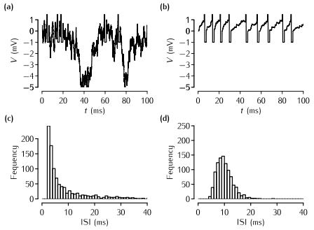
(a) The Stein (1965) model with balanced excitation and inhibition. The time course of the voltage over 100 ms of an integrate-and-fire neuron that receives inputs from 300 excitatory synapses and 150 inhibitory synapses. Each synapse receives Poisson spike trains at a mean frequency of 100 Hz. The threshold is set arbitrarily to 1 mV, the membrane time constant of the neuron is 10 ms, and there is a refractory period of 2 ms. Each excitatory input has a magnitude of 0.1 of the threshold, and each inhibitory input has double the strength of an excitatory input. Given the numbers of excitatory and inhibitory inputs, the expected levels of excitation and inhibition are therefore balanced. (b) The time course of a neuron receiving 18 excitatory synapses of the same magnitude as in (a). The output firing rate of the neuron is roughly 100 Hz, about the same as the neuron in (a), but the spikes appear to be more regularly spaced. (c) An ISI histogram of the spike times from a sample of 10 s of the firing of the neuron in (a). (d) An ISI histogram for the neuron shown in (b).
Simulation environment:
Notes
To reproduce the data behind panel (a) and (c):
- In the RunControl window click on Init&Run
- A trace of the membrane potential appears in the top window and at the end of the simulation the histogram appears in the lower window.
To reproduce the data behind panel (b) and (d):
- In the Parameters window change NE to 18 and change NI to 150.
- In the RunControl window click on Init&Run.
You can also explore the effect of changing the strength of the excitatory and inhibitory inputs by changing JE and JI in the Parameters window.
Download: